Take a look at this:
This is a triangulation of a set of random points, such that all the points are connected to one another, all of the faces are triangles, and the edges include the convex hull of the points.
I would like to claim that this is not a very “good” triangulation. This algorithm tends to produce lots of long, slivery triangles, and a really uneven distribution of edge counts across different vertices – some vertices have way more edges than they need to.
Here’s a different triangulation. These are the exact same points, but I triangulated them smarter:
Isn’t that better? (Click to compare!)
Depending on your dice rolls you might still have a few slivers, usually around the outer perimeter, but I’m willing to bet that it’s a noticeable improvement over the first attempt.
This triangulation is called the Delaunay triangulation, and I would like to claim that it is a very good triangulation. It is, in fact, the best possible triangulation, for some definitions of “best.”
Why should I, a busy person with important responsibilities, care about triangles?
Okay, right, good question. You’ve made it this far in life without triangulating anything; why should you start now?
There are some obvious applications of triangulation algorithms in computer graphics, where everything is made out of triangles, but you knew that already and you are still unmoved.
Let’s try something else.
One textbook example of a non-graphics application of the Delaunay triangulation is interpolating spatial data.
Pretend, for a moment, that you’re a surveyor, and you’ve just finished measuring the elevation of a bunch of discrete points in some area. You sling your weird tripod thingy over your shoulder, and get ready to leave for the first vacation you’ve been able to take with your son since Terence left – when your boss appears at your door.
“What’s the elevation three clicks south of the north ridge, or however surveyors talk?” she asks.
You glance down at the oversized roll of mapping paper (?) on your desk, but you already know what you’ll find: you didn’t take a measurement three clicks south of the north ridge. But you did measure a few points nearby. Perhaps, you think, I can construct a triangulation of these points, and then map it to a three-dimensional mesh, and use that to interpolate the elevations between nearby points.
You call your son to tell him that you’ll be a little late – it’s 1998 in this situation; texting isn’t a thing yet – and get to work.
But after the montage ends, you look upon your work, and find… oh.
Well that’s not going to work.
You pick up the phone to make another difficult call, but as your finger hovers over the rotary dial, you suddenly remember an incredibly long blog post that you read once – or that you will read; it’s 1998 still; this blog post hasn’t been published yet; it’s too late to change it now; just go with it – and you put the receiver back on the cradle.
And then you construct the Delaunay triangulation of the exact same points:
(Click to add sheep, obviously.)
You shoot your boss a quick fax and get ready to hit the road. But as you stand up to leave, you see her standing in your doorway yet again.
“I just got off the corded phone with President Clinton,” she says. “Your triangles are so good that he’s appointing you Surveyor General. When you get back from vacation, I’ll be reporting to you.”
So that’s the first reason to learn about Delaunay triangulation.
Here’s another one: did this idea of interpolating “nearby” points remind you of anything else? Perhaps… the Voronoi diagram? If so, you are smart and attractive: one easy way to construct the Voronoi diagram is to calculate the Delaunay triangulation, because the Delaunay triangulation is the dual of the Voronoi diagram.1 Which is neat if you know what “dual” means. If you don’t know what dual means, keep reading! We’re going to talk about duals a lot later on.
So those are like… some good reasons to learn about Delaunay triangulations.
But I did not learn about Delaunay triangulations for a good reason.
I learned about Delaunay triangulations for the dumbest reason you can possibly imagine.
Here, it’s easier if I just show you.
I heard the phrase “smash that subscribe button” once, and after a brief moment’s existential crisis as I realized that I am now old enough that I recoil from the parlance of youth, I thought it would be funny to make a subscribe button that you could smash.2
In case you already smashed that one, here’s another:
It’s kinda fun, right?
I’ve been meaning to add an email subscription button to my website for a while, and the thought of implementing this visual gag was enough of an incentive for me to actually get around to it.
I thought that a decent way to randomly fracture a shape into polygons would be to compute the Gabriel graph of a set of random points inside the button.3 And the easiest way to compute the Gabriel graph is to compute the Delaunay triangulation and then remove a few edges from it. So that’s why I started looking into this in the first place.
But it was pretty hard! Although it’s easy to find explanations of Delaunay triangulation algorithms in vague, mathematical terms, I couldn’t find very many resources describing how to actually implement them. Like, I’m trying to construct an infinitely large triangle, but my computer keeps catching on fire – what do I do now, Professor Triangle?
So this is going to be an explanation for the “working programmer.” I’m going to describe a deceptively simple algorithm for Delaunay triangulation, and then the actual edge-cases that you have to think about when you try to implement it. And I’m going to do it without ever using the word “manifold.”
Starting… now.
What is a Delaunay triangulation?
The Delaunay triangulation is the triangulation that “maximizes the minimum angle in all of the triangles.”
Here’s, it’s easier if we look at an example:
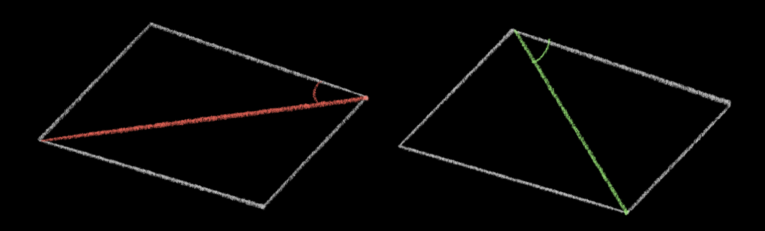
Obviously all the angles of a triangle add up to 180°, but the triangles on the left get there with two very acute angles and one obtuse angle, while the triangles on the right have only acute angles – but they are not as acute as the acute angles on the left.
These are the only two triangulations of these four points, so the one on the right is the optimal triangulation according to our criteria – in other words, it is the Delaunay triangulation of this point set.
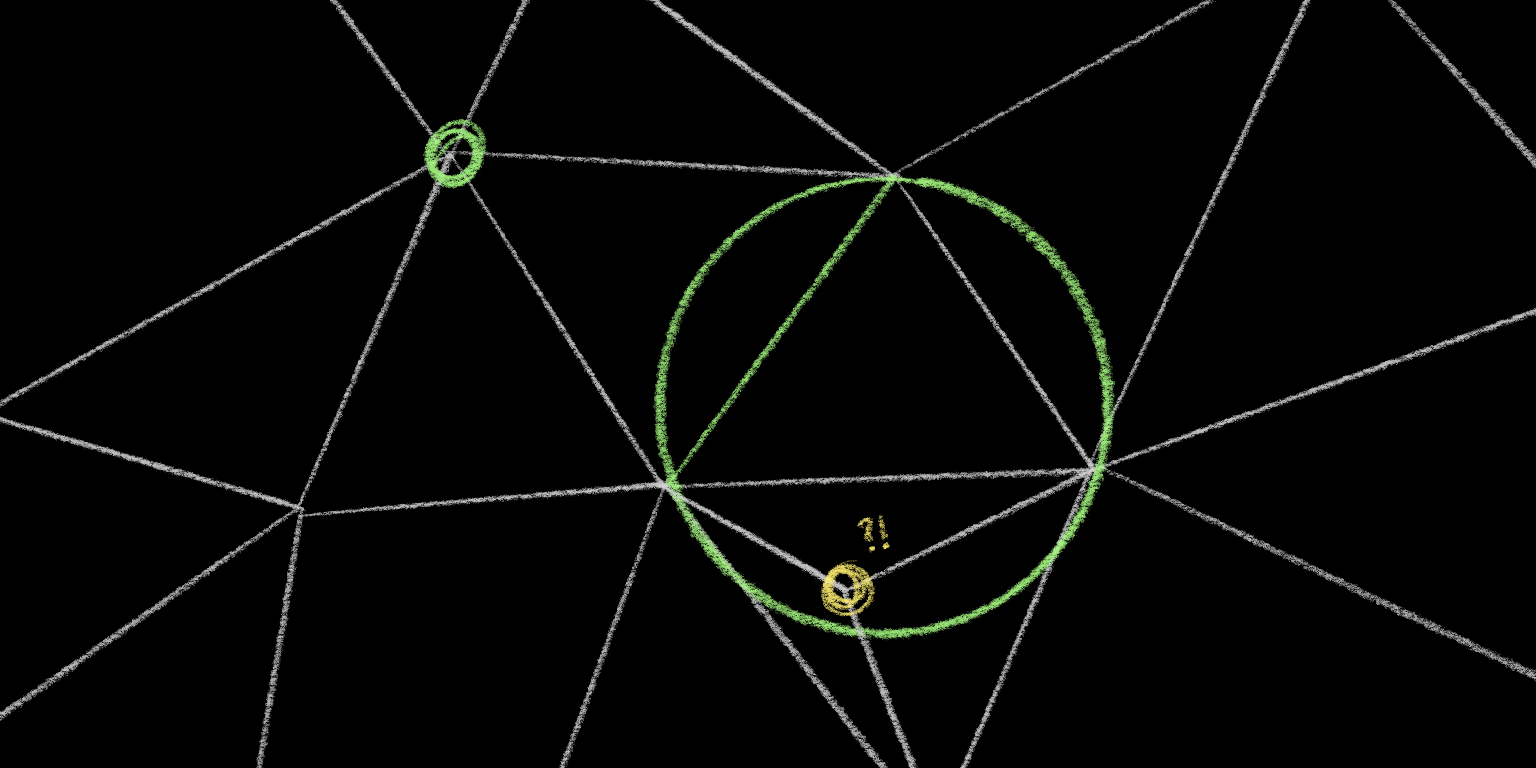
Here’s an equivalent, but more useful definition: the Delaunay triangulation is the triangulation such that, if you circumscribe a circle around every triangle, none of those circles will contain any other points.
(Click or tap to pause that, if the flashing is distracting.)
I’m going to make a potentially surprising claim: this is the only such triangulation of these points that satisfies that property. If you were to change any single edge – rearrange any of these triangles in any way – you would have at least one point inside another triangle’s circle territory.4
It’s worth noting that this is a global property of the triangulation – it’s a statement about every triangle and every point at the same time. Global properties are expensive to check and expensive to change, so we’d much rather focus on a local property during our algorithm.
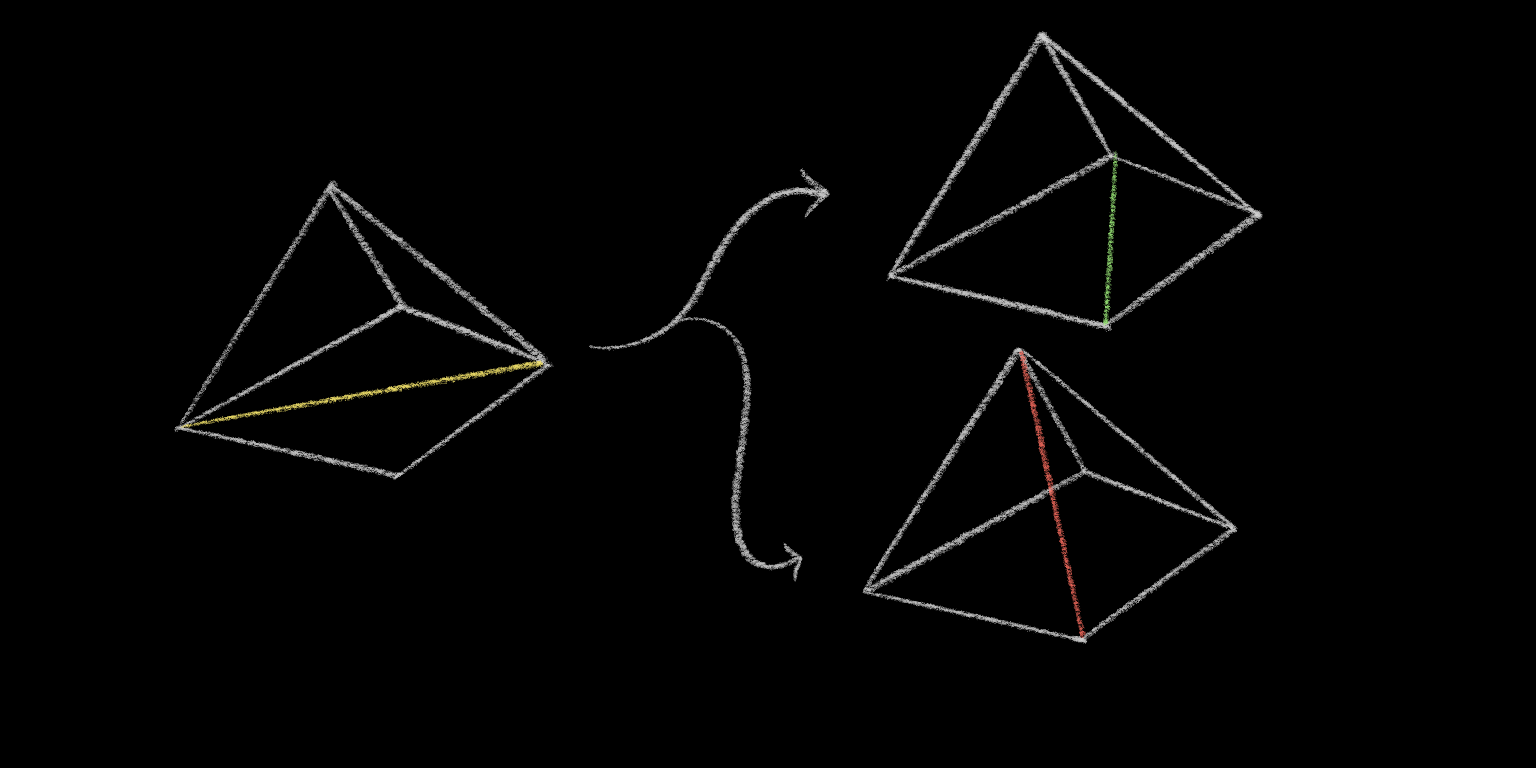
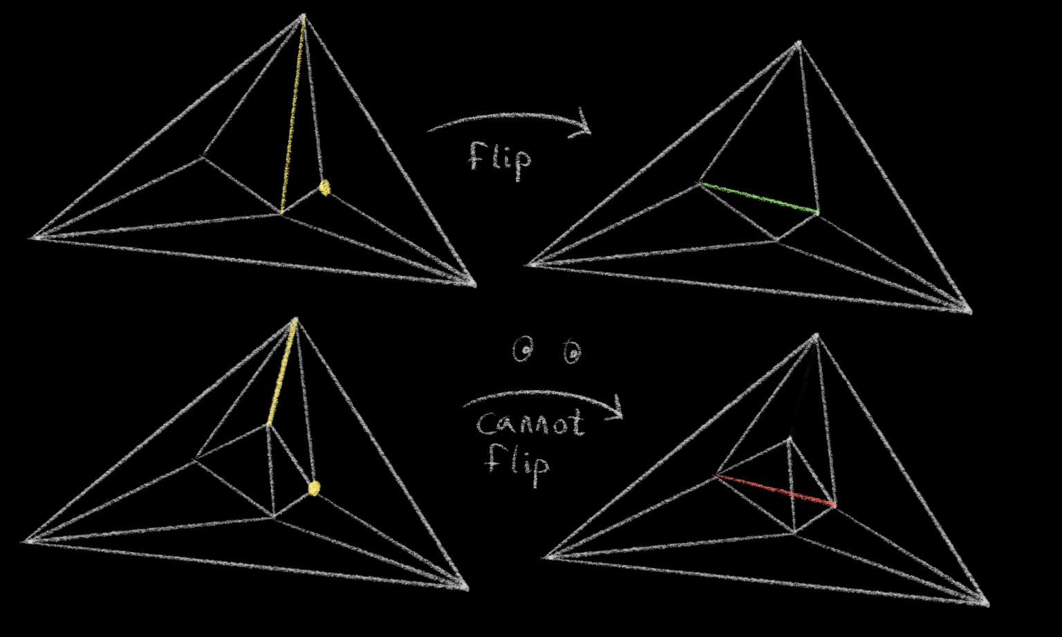
So let’s consider a single edge on the triangulation. Specifically an interior edge, not an edge around the perimeter.
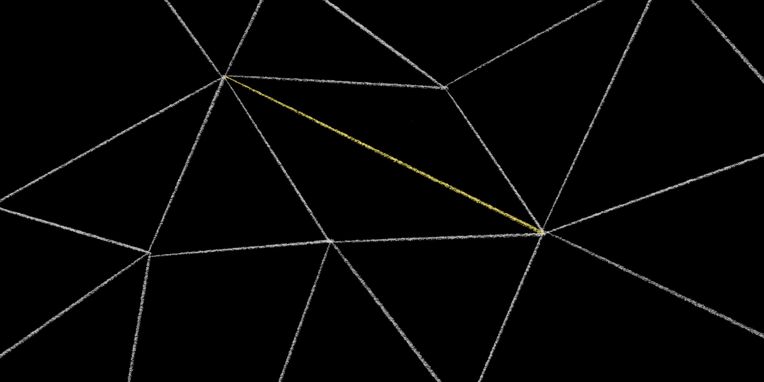
There are two triangles on either side of this edge. Pick one at random, and draw a circle around it.
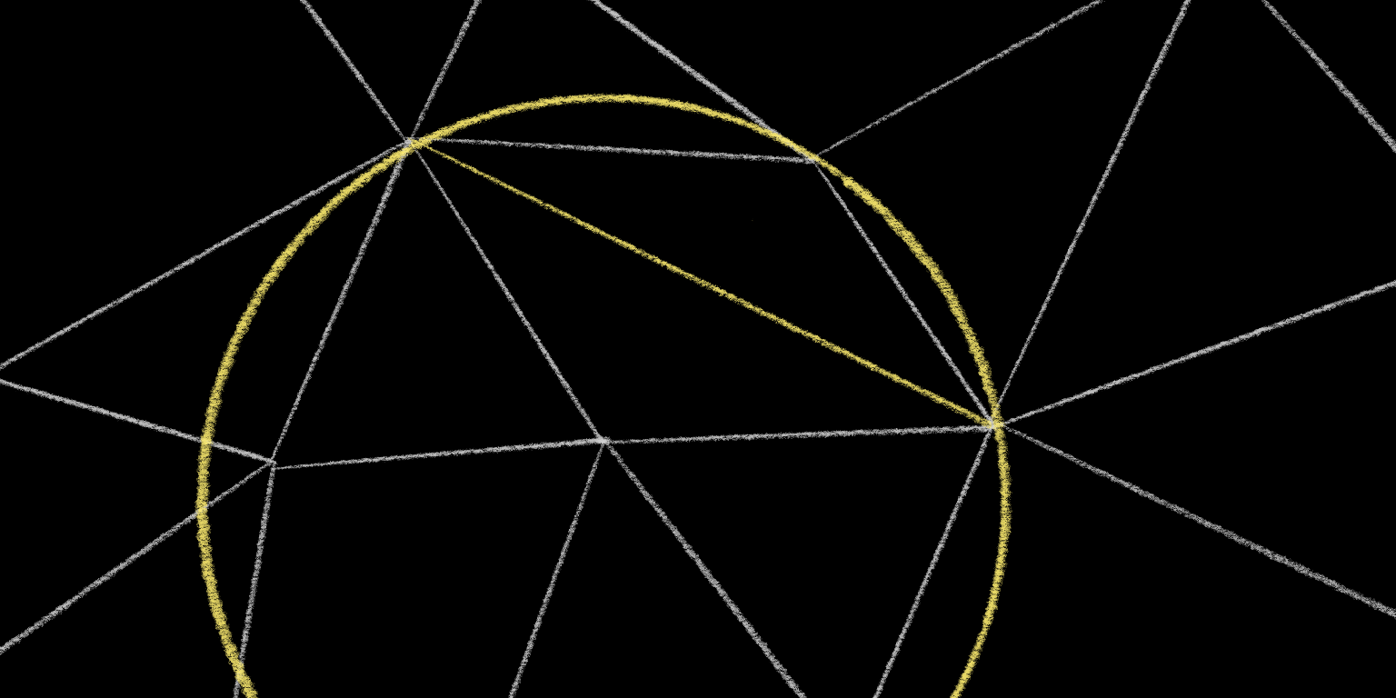
Now check if the tip of the other triangle adjacent to this edge lies inside or outside of this circle. If it lies outside the circle, then this edge is “locally Delaunay.” If it lies inside the circle, then the edge is not “locally Delaunay.”
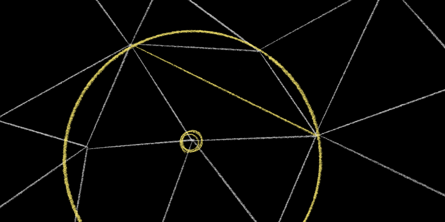
In this case, the point is very much inside the circle, so we know that this is a bad edge. But if we then flip the edge so that it connects the other two points of our quadrangle, then this flipped edge is guaranteed to be locally Delaunay:

Notice that there might be other points that lie inside this circle that we didn’t check.
Because we only checked local Delaunayness, which is only concerned with this one particular point on the other side of the edge.
But here’s the trick: as long as every edge of the triangulation is locally Delaunay, the entire triangulation is a Delaunay triangulation. If this were a computational geometry class we’d spend the next ten minutes proving that statement, but for now I’ll just ask you to trust me on it.
Okay. So now that we know these things, we can start to imagine an algorithm. We want to make a triangulation such that all edges are “locally Delaunay.” If we started with any triangulation, we could just loop over all the edges, flipping any edges that are not locally Delaunay, and repeat until we don’t find any edges that need to be flipped.
Would that work? Or is there a chance that we’d get into an infinite loop, repeatedly flipping and un-flipping edges due to some weird complicated cycle? It’s not obvious to me that this is the case, but apparently it does work – but only in two dimensions! – and will eventually terminate after O(n2) flips.
But we can do better.
Guibas & Stolfi’s incremental triangulation algorithm
There are several “better” algorithms, but the one I’m going to describe comes from Guibas & Stolfi’s seminal 1985 page-turner “Primitives for the Manipulation of General Subdivisions and the Computation of Voronoi Diagrams."
It’s an incremental algorithm, which means that you can start triangulating something even if you don’t know all of the points up-front, or you can use it to add new points to an existing Delaunay triangulation without having to re-triangulate it from scratch.
It’s the most popular algorithm that I came across, probably because it’s very easy to understand it conceptually.5 But for all the explanations of it that exist on The Internet, I could not find a single resource that actually explains it in sufficient detail that you could go write the code for it! I had to cobble an understanding together from the original paper, lecture notes, actual lectures on YouTube – and ultimately by sitting down and working out some details myself.
So I’m going to try to correct that here.
But before I describe the algorithm, let me show it to you. You already know about “locally Delaunay” edges, which is the only real trick here – see if that’s sufficient to work out what the algorithm is doing.
Click to start/stop the animation, or drag the scrubber to move frame-by-frame.
Okay, so at a high level, the algorithm is deceptively simple:
Start with a single “infinitely large” triangle – although note that, in tonight’s performance, infinitely large triangle will be portrayed by appropriately-sized finite triangle, in order to make the visualization easier to understand.
Next, loop through your points, and add them into the triangulation one-by-one. Notice that our single giant triangle is, trivially, a valid Delaunay triangulation, which is a precondition that will hold at the beginning of every iteration.
Every time you add a point, split the triangle that contains it into three new triangles, and then check the locally Delaunay condition. You know that you started with a valid Delaunay triangulation, so you only have to look at the edges immediately surrounding the point that you added – the rest of the edges are already good. Flip any edges that are not locally Delaunay, and then check the edges adjacent to those flipped edges, because the act of flipping might have made them invalid. Then once you’re done checking and potentially flipping all of the “dirty” edges, you’re done! You have a valid Delaunay triangulation once again, and you’re ready for the next point.
Once you run out of points, just remove the infinitely large outer triangle – and the edges connected to it – and you have your final triangulation.
Easy, right?
no; you’ve used the phrase “deceptively simple” twice already
Right. So that explanation might be sufficient if you’re a mathematician, but if you actually tried to write the code for this, you’ll quickly run into questions like the following:
- I can’t actually construct an infinitely large bounding triangle – is it okay if I just construct a triangle large enough that it contains all of my points?
- How am I supposed to find the triangle that contains my new point?
- What if the new point lies on the edge of an existing triangle?
- How am I supposed to do this “circle test” in the first place?
- What edges do I actually need to check, once I’ve added my new edges?
- Wait, how do I “flip” edges?
- Wait, how do I even model edges? How do you even represent triangulations on a computer? I thought I could just model this as a graph, with vertices and edges and pointers, but it seems like I need to keep track of faces as well, and somehow this is a fundamentally different sort of thing than I’ve ever encountered before?
Well, those were the questions I had, anyway.
And now I have the answers.
Let’s start with (3) because (3) is easy: if a point falls on an existing edge, you want to delete the edge, then create four new triangles instead of the normal three. The odds of this happening in a randomly generated point set is astronomically low, so here’s a hand-picked example that demonstrates what this looks like:6
This prompts a new question – “how do I delete an edge?” – but we’ll answer that at the same time we figure out how to flip edges.
The rest of the questions have… slightly more involved answers.
So let’s start with a fun one.
How to check if a point is inside a circle
It’s very easy to check if a point is in a circle if you know the circle’s radius and center – you compare the distance from the point to the center of the circle against the circle’s radius.7 But we don’t know the circle’s center or radius; we only know these three points on its circumference.
Now, we could solve for the circle’s center and radius. There are many techniques for doing this, but it’s relatively expensive – we don’t want to be taking square roots or doing any floating-point division here, because we’re going to be doing this point-in-circle test a lot.
Instead, Guibas & Stolfi describe a really interesting technique that, when I first encountered it, made absolutely no sense to me.
Their technique is to calculate the determinant of this 4x4 matrix:
| Ax | Ay | Ax2 + Ay2 | 1 |
| Bx | By | Bx2 + By2 | 1 |
| Cx | Cy | Cx2 + Cy2 | 1 |
| Px | Py | Px2 + Py2 | 1 |
(Where (A, B, C) are the points that define the circle, and P is the point to test.)
If the determinant is positive, the point is inside the circle. If it’s negative, the point is outside of the circle. If the determinant is zero, the point also lies on the circle.
Okay what.
So I don’t expect this to make sense to you. It didn’t make sense to me when I first heard it. But I’m going to try to explain it, in a little more detail than Guibas & Stolfi explain it.
First off: we have a bunch of 2D points. We’re going to transform them into 3D points, by saying:
z = x2 + y2
This gives us a bunch of points in 3D. Specifically, it projects these points upwards onto this weird parabaloid shape:
(Click and drag the points to move them around.)
Okay. So that’s… something.
We know that three points in 3D space uniquely determine a plane (unless the points are co-linear). Planes seem simpler than circles. So you can maybe see how this is a step in the right direction. Let’s draw the plane:
Now, there’s something very interesting about this plane: if we look at the points where it intersects our parabaloid, we can see that it forms some kind of ellipse shape.
But if we look at it straight down from the top, we can see that the ellipse projects a perfect circle onto the XY plane.
Specifically, the circle that passes through all of our original points. So if we project the intersection of this plane with the parabaloid back down onto the XY plane, we get the circle that we actually care about:
Okaaaaay. So we’ve established a correspondence between this weird parabaloid shape and the circle in question. But let’s not forget why we’re doing this: we want to check if a point is inside this circle.
So let’s add another point.
Drag it around a little bit, and hopefully you can see where we’re going with this.
When we project that point upwards to the parabaloid, the point where it hits is either going to lie “under” or “over” our plane. And you can see that it’s going to hit “under” the plane exactly when the point is in the circle.
Okay! So this is interesting. This already suggests a very simple circle test algorithm: instead of finding the equation for the circle, find the equation for this plane. Then project our point upwards to both the plane and the parabaloid. If the projection up to the parabaloid is lower than the projection to the plane, then it’s inside the circle.
It’s easy to find the equation for a plane. Given three points (A, B, C), all we have to do is find any vector orthogonal to the plane, which we can do by taking the cross product of any two vectors on the plane:
N = (B - A) ⨯ (C - A)
And that, combined with any one of our original points, gives us an equation for the plane:
Nx(x - Ax) + Ny(y - Ay) + Nz(z - Az) = 0
Which we can use to solve for z, giving us a function of x and y:
plane(x, y) = -(Nx(x - Ax) + Ny(y - Ay)) / Nz + Az
Okay, neat. Now if you recall our parabaloid equation:
parabaloid(x, y) = x2 + y2
Then all we have to do is compare the value of these two functions, and we have our circle test:
contains(x, y) = parabaloid(x, y) < plane(x, y)
Okay. That makes sense, right?
But that’s not what Guibas & Stolfi did.
Notice how there are no weird complicated matrices involved in that calculation. Yes, I did take a cross product, but that’s a pretty small amount of linear algebra to stomach compared to the determinant of a 4x4 matrix.
So.
Let’s return to Guibas & Stolfi’s solution. Remember that they propose calculating the determinant of this matrix:
| Ax | Ay | Ax2 + Ay2 | 1 |
| Bx | By | Bx2 + By2 | 1 |
| Cx | Cy | Cx2 + Cy2 | 1 |
| Px | Py | Px2 + Py2 | 1 |
Hmm.
I can understand 3x3 matrices. I’ve made my peace with them. I can think of them as transformations of 3D points to other 3D points. I’ve even almost, sort of, reluctantly made peace with determinants: I can understand the determinant of a 3x3 matrix as the rate by which it scales volumes when you transform shapes with it.
4x4 matrices… I have no intuition for them. I would expect the determinant of a 4x4 matrix to be some kind of scaler of hypervolumes. But since it’s only barely four-dimensional – all values on the “W axis” are 1 – we can intuit that we’re probably just dealing with plain volumes again.
And in fact that’s correct: this determinant is actually the (oriented!) volume of the parallelepiped that has these four points as corners.
Whoa, that’s… a lot. That’s kind of hard for me to parse. But in the same way that a parallelogram consists of (2! = 2) identical triangles, a parallelepiped consists of (3! = 6) identical tetrahedra. Let’s focus on just one of them:
So I have two things to say about this.
First off: notice that sometimes the tetrahedron is “inside out:” it has a negative volume, which I represent by changing the color of the wireframe. The crux of the point-in-circle test is checking the sign of that volume, and you can see if you move the free point around that it does invert when the free point passes into or out of the circle.
But! If you move the other points around, you can change whether positive or negative means “point in circle” or “point outside of circle.” Try it: swap the location of any two points on the circle, and watch as the sign flips, even though the circle remains the same.
This is because the orientation of the tetrahedron depends not only on the position of the free point relative to the three circle points, but also the orientation of the three circle points relative to one another. So this test only works if you make sure that you list the points (A, B, C) in a clockwise order. If you list them in counterclockwise order, the circle will be “inside out,” and the test will give you the wrong answer.
Which is pretty annoying.
So… I don’t like this test as much as the plane test in general. It seems more expensive8 to calculate the determinant than to calculate the equation of the plane, and it seems really annoying that you have to be careful that you provide the points in the right order or you’ll get the wrong result.
This isn’t actually a problem for us, because we’ll be use a fancy data structure for storing edges that ensures we can only provide points in the correct order.
Anyway.
Second thing:
A more obvious way to calculate the volume of a parallelepiped is to pick one point as the origin, and then to write the other three points relative to this origin. Then we have three points in three dimensions, which we can express as a square matrix:
| Ax - Px | Ay - Py | (Ax2 + Ay2) - (Px2 + Py2) |
| Bx - Px | By - Py | (Bx2 + By2) - (Px2 + Py2) |
| Cx - Px | Cy - Py | (Cx2 + Cy2) - (Px2 + Py2) |
And the determinant of this matrix gives us the volume of the same parallelepiped as before, but in the simple straightforward way that we remember from that one linear algebra class we almost passed.
Now, the determinant of this matrix is exactly equal to the determinant of the 4x4 matrix that you get by padding each point with a 1. They’re just two ways of saying the same thing. You could verify that algebraically, but I feel like there’s probably some intuitive explanation of this fact, and understanding why this is would lead to a better understanding of determinants in general and maybe teach me how to use higher dimensional matrices to more easily perform calculations in lower dimensions. Like in some way the fourth point we added sort of acts as a new origin? At least in this particular case?
But look: I have to stop somewhere, or I’m never going to finish this blog post. And this is the place I decided to stop exploring Guibas & Stolfi’s point-in-circle test.
For now.
Back to the triangulation
Where were we?
- I can’t actually construct an infinitely large bounding triangle – is it okay if I just construct a triangle large enough to contain all of my points?
- How am I supposed to find the triangle that contains my new point?
What if the new point lies on the edge of an existing triangle?How am I supposed to do this circle test in the first place?- What edges do I actually need to check, once I’ve added my new edges?
- Wait, how do I “flip” edges?
- Wait, how do I even model edges? How do you even represent triangulations on a computer? I thought I could just model this as a graph, with vertices and edges and pointers, but it seems like I need to keep track of faces as well, and somehow this is a fundamentally different sort of thing than I’ve ever encountered before?
Okay. Let’s talk about (7) next, because you’re losing steam and it’s very interesting. The other questions are pretty specific to this one algorithm that you don’t actually care about – although I appreciate how polite you are being – but this one is broadly applicable to lots of graph-related, mesh-related, and computational geometry-related problems.
The quad-edge data structure
Okay, so you know how to represent a graph, right? You have some Node or Vertex objects, and you have some Edge objects, and vertices have pointers to their edges and edges have pointers to their vertices. Or you store an adjacency matrix; that’s a thing I’ve heard of.
This works great when you’re dealing with graphs in the abstract – if all you’re doing is Dijkstra’s algorithm or finding biconnected components or whatever, this simple representation works fine.
But in this case we’re also concerned with faces – when we flip an edge, we need to know the specific faces we’re flipping it on, so we don’t do something illegal:
The obvious-to-me way to do this is to add another object to the mix: model Faces explicitly, and have edges keep track of the faces they’re a part of, and every time you change anything about the graph you have to make sure to keep the faces and edges and vertices all in sync. I actually tried this, during my first forays into triangulation. It was awful. Just a case study on how denormalization will ruin your day. We’re not going to do that.
Fortunately, Guibas & Stolfi describe a very clever alternate representation called the “quad-edge” data structure.
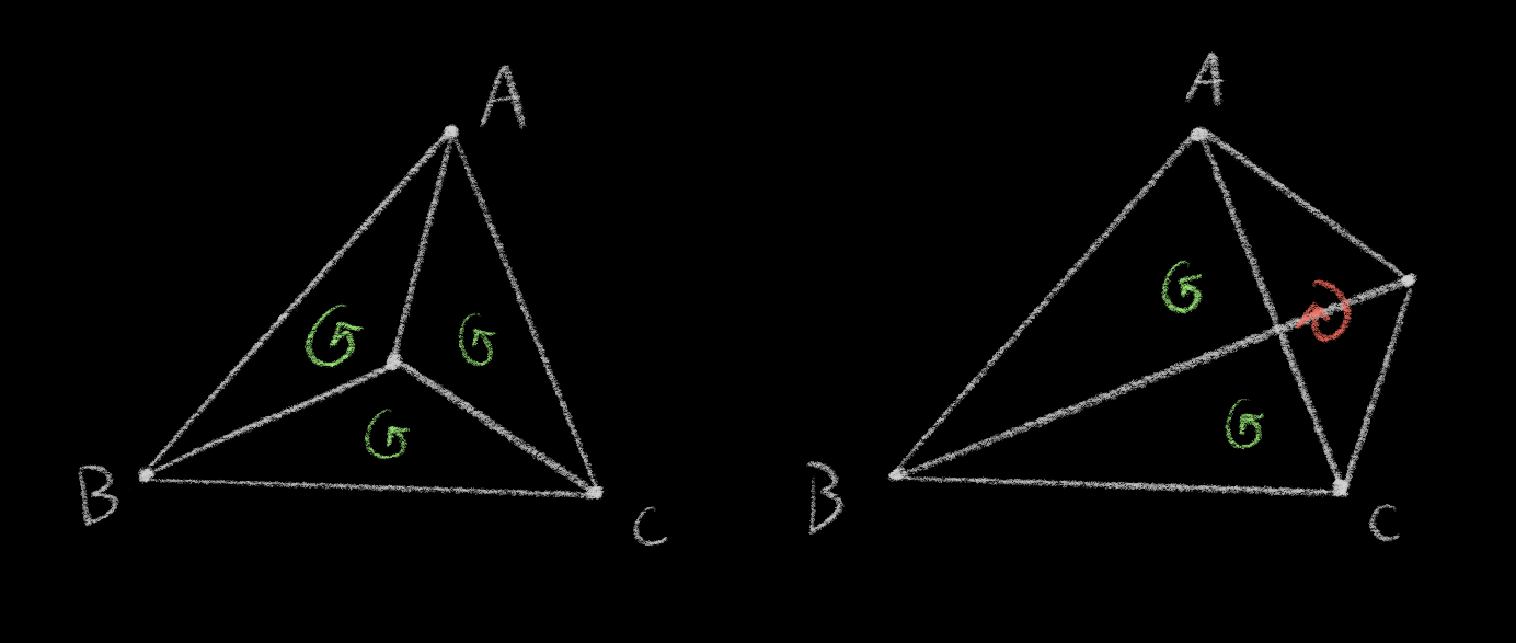
To understand the quad-edge structure, you first have to understand the idea of the dual of a graph. Very loosely, if you take a drawing of a graph9 and put a vertex in the middle of every face, and then connect all of the adjacent “face-vertices” with edges, you’ll have the dual graph. It’s easier to understand with a picture:

That’s actually a simplification – I’m missing one face from all of those graphs: the outer face, the inside-out face bounded by the outside of the graphs. Here are the actual duals:
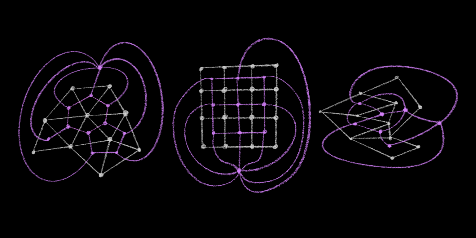
But since that is a mess to look at, I will instead adopt the following shorthand, and trust that you can imagine the outer face:

Okay, so duals. Neat. Who cares?
Well, the high level idea of the “quad-edge” structure is that you break every undirected edge A <-> B of your mesh into four separate directed edges: one that represents A -> B, one that represents B -> A, and two others that represent the directed dual edges of the faces on either side of the edge. So for each undirected edge on our graph, we would have four directed edges like so:
So the quad-edge structure represents the structure of a graph and its dual at the same time: a quad-edge is just a list of these four directed edges.
I was very confused about this when I was reading Guibas & Stolfi.10 They never give a type definition for quad-edges, and they describe operations on quad-edges that don’t actually apply to quad-edges – they apply to the directed edges that comprise quad-edges. Guibas & Stolfi call these “quad-edge refs,” but because that is confusing and clumsy I will call them “quarter-edges” from here on out.
The paper is hard to follow sometimes because it uses the term “edge” a lot, which could mean one of three different things:
- A logical edge on a graph – that is, the normal sense of the word.
- A “quad-edge,” which represents a single logical edge, and consists of four individual parts.
- A “quarter-edge” (my term) or “quad-edge ref” (their term), which is one of the individual parts of a quad-edge.
Now here’s the trick: whenever they say “edge” or “quad-edge,” they actually mean “quarter-edge.” For example:
The second operator is denoted by
Splice[a, b]and takes as parameters two edgesaandb, returning no value.
Splice is actually an operation on quarter-edges. If you try to make sense of it as an operation on quad-edges, you will have a bad time and be very confused.
Anyway.
Digression over.
Guibas & Stolfi don’t prescribe a concrete representation, but here’s a straightforward way11 to represent the quad-edge as they describe it:
typedef struct {
    quarter_edge refs[4];
} quad_edge;

typedef struct {
    quad_edge *my_quad_edge;
    int my_index;

    quad_edge *next_quad_edge;
    int next_index;

    void *data;
} quarter_edge;

quarter_edge *rot(quarter_edge *edge) {
    return edge->my_quad_edge->refs[(edge->my_index + 1) % 4];
}

quarter_edge *sym(quarter_edge *edge) {
    return edge->my_quad_edge->refs[(edge->my_index + 2) % 4];
}

quarter_edge *tor(quarter_edge *edge) {
    return edge->my_quad_edge->refs[(edge->my_index + 3) % 4];
}

quarter_edge *next(quarter_edge *edge) {
    return edge->next_quad_edge->refs[edge->next_index];
}
rot (“rotate”), sym (“symmetric edge”), and tor (“rotate the other way”) are functions that bring you to the other three quarter-edges on the same QuadEdge. next is a pointer that allows you to navigate around to adjacent QuadEdges in the structure. (We’ll come back to this in a minute.)
So you can see that a quad-edge isn’t really a thing; it’s just a bundle of four other things. And in fact I think it’s much simpler if we just pretend that quad-edges don’t exist, and define everything in terms of quarter edges:
typedef struct {
    void *data;
    quarter_edge *next;
    quarter_edge *rot;
} quarter_edge;

quarter_edge *rot(quarter_edge *edge) {
    return edge->rot;
}

quarter_edge *sym(quarter_edge *edge) {
    return edge->rot->rot;
}

quarter_edge *tor(quarter_edge *edge) {
    return edge->rot->rot->rot;
}
Whenever we create these, we can just create four of them at a time, and set their rot pointers in a cycle such that edge == edge->rot->rot->rot->rot. This representation is slightly less efficient, but it’s much simpler, especially when we start manipulating it.
Okay, with that out of the way: what is next?
next points to a quarter-edge that:
- Has the same starting point (be it a vertex or a face) as this quarter-edge.
- Lies immediately counter-clockwise of this quarter-edge.
This is all a little abstract, so let’s make it concrete. This is a little demo that lets you play with the quad-edge structure: the “current” edge is highlighted in yellow, and you can traverse the structure by pressing WASD (if you have a keyboard).
WsymAtorSnextDrot
Notice that the WAD keys will only move you between each of the four quarter-edges of the current quad-edge, while S will allow you to move to other edges.
(Notice that, because the outer face is “inside out,” pressing S while on the outer face will actually move clockwise around the perimeter.)
You can compose these operations predictably to navigate around. For example, to go to the “previous” edge that shares the same point – to navigate clockwise, in other words – press DSD. To navigate around the triangle to the left of the current edge, press ASD repeatedly. To navigate around the triangle to the right of the edge, press WS.
We’ll be doing some of these a lot, so we’ll give them names:
prev = rot.next.rot
lnext = tor.next.rot
The last thing that I didn’t explain is the data pointer.
The data pointer stores arbitrary information about the vertex or face at the beginning of each directed quarter-edge. For our purposes, we’ll use data to store the actual location in space of each vertex, and we won’t store anything on faces. So note that, since there are multiple directed edges out of each vertex, all quarter-edges that you reach by traversing the next pointers – by pressing S, in the demo – will have identical data pointers.
One thing that’s a little weird about this representation is that each “directed edge” doesn’t actually store anything about its destination. Its data pointer only contains its origin, and the destination of the edge is implicit from its sibling quarter-edges. Specifically, each quarter-edge represents a directed edge from edge.data to edge.sym.data.
We’ll refer to edge.sym.data a lot, so I’m going to give it a shorthand as well:
dest = sym.data
So: that’s it! That’s the structure.
How do we… use it?
Well first we need to be able to create quarter-edges – which we always do in groups of four:
function makeQuadEdge(start, end) {
  const startEnd = new QuarterEdge();
  const leftRight = new QuarterEdge();
  const endStart = new QuarterEdge();
  const rightLeft = new QuarterEdge();

  startEnd.data = start;
  endStart.data = end;

  startEnd.rot = leftRight;
  leftRight.rot = endStart;
  endStart.rot = rightLeft;
  rightLeft.rot = startEnd;

  // normal edges are on different vertices,
  // and initially they are the only edges out
  // of each vertex
  startEnd.next = startEnd;
  endStart.next = endStart;

  // but dual edges share the same face,
  // so they point to one another
  leftRight.next = rightLeft;
  rightLeft.next = leftRight;

  return startEnd;
}
That represents a single edge that cuts through a single face – the face on the left and right of it are the same, and it exists on its own, connected to nothing. Guibas & Stolfi have a nice illustration of what this means topologically:
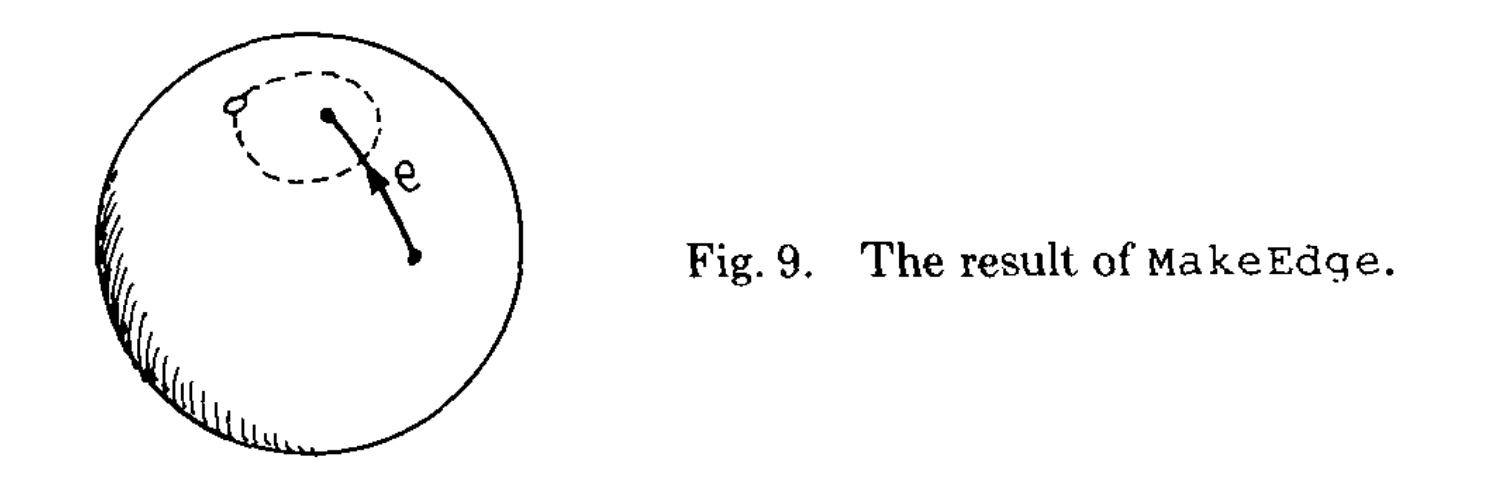
Reprinted by permission of the Association for Computing Machinery
Simple.
The next operation lets us connect edges together, or tear them apart. It’s called splice, and it’s probably just as simple. Let’s see how Guibas & Stolfi explain it:
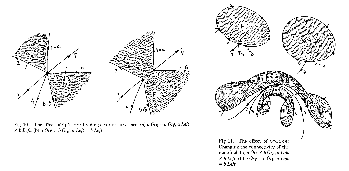
Reprinted by permission of the Association for Computing Machinery
Aaaah! Oh dear. Topology is happening to us, and it doesn’t feel good.
But the implementation is so simple:
function splice(a, b) {
  swapNexts(a.next.rot, b.next.rot);
  swapNexts(a, b);
}

function swapNexts(a, b) {
  const anext = a.next;
  a.next = b.next;
  b.next = anext;
}
We’re just swapping a couple of pointers – it seems like it should be simple to understand. But it’s very difficult to intuit the effect that this actually has on our mesh.
Let’s use it in a sentence. splice is a low-level primitive operation, and we’ll never actually call it directly in our algorithm. Instead, we’ll use it to build higher-level operations, and seeing how these operations use splice under the hood is probably the best way to gain intuition for how it works.
So the first thing we’ll need to do is construct a bounding triangle:
function makeTriangle(a, b, c) {
  const ab = makeQuadEdge(a, b);
  const bc = makeQuadEdge(b, c);
  const ca = makeQuadEdge(c, a);

  splice(ab.sym, bc);
  splice(bc.sym, ca);
  splice(ca.sym, ab);

  return ab;
}
Then we’ll need to know how to add new edges:
function connect(a, b) {
  const newEdge = makeQuadEdge(a.dest, b.data);
  splice(newEdge, a.lnext);
  splice(newEdge.sym, b);
  return newEdge;
}
And how to remove edges:
function sever(edge) {
  splice(edge, edge.prev);
  splice(edge.sym, edge.sym.prev);
}
And how to insert new points into an existing polygon:
function insertPoint(polygonEdge, point) {
  const firstSpoke = makeQuadEdge(polygonEdge.data, point);
  splice(firstSpoke, polygonEdge);
  let spoke = firstSpoke;
  do {
    spoke = connect(polygonEdge, spoke.sym);
    spoke.rot.data = null;
    spoke.tor.data = null;
    polygonEdge = spoke.prev;
  } while (polygonEdge.lnext !== firstSpoke);
  return firstSpoke;
}
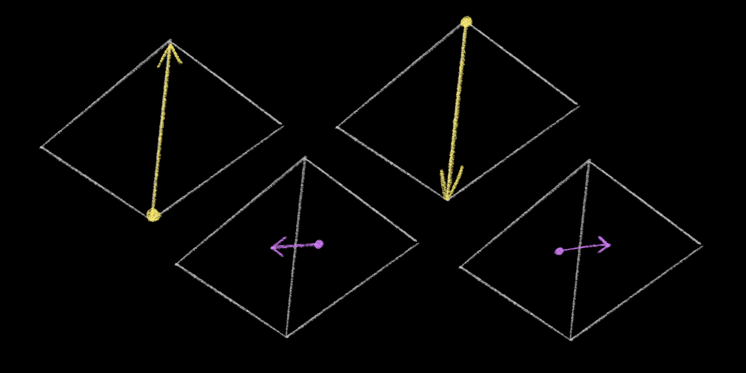
And lastly we’ll need to “flip” the diagonal edge of a quadrangle.
function flip(edge) {
  const a = edge.prev;
  const b = edge.sym.prev;
  splice(edge, a);
  splice(edge.sym, b);
  splice(edge, a.lnext);
  splice(edge.sym, b.lnext);
  edge.data = a.dest;
  edge.dest = b.dest;
}
And that’s it! Those are the only operations we need.
I think the easiest way to understand splice is to work through these high-level operations and convince yourself that this series of pointer updates gives you the QuarterEdge structure that you want. But also: you can just trust me. You aren’t actually trying to implement this.
are we done yet
Almost!
- I can’t actually construct an infinitely large bounding triangle – is it okay if I just construct a triangle large enough to contain all of my points?
- How am I supposed to find the triangle that contains my new point?
What if the new point lies on the edge of an existing triangle?How am I supposed to do this circle test in the first place?- What edges do I actually need to check, once I’ve added my new edges?
Wait, how do I “flip” edges?Wait, how do I even model edges? How do you even represent triangulations on a computer? I thought I could just model this as a graph, with vertices and edges and pointers, but it seems like I need to keep track of faces as well, and somehow this is a fundamentally different sort of thing than I’ve ever encountered before?
Now that you understand the quad-edge/quarter-edge structure, we can talk about (2). It’s clever! It’s not what you’re expecting!
triangle where
So in order to add a new point to your mesh, you first need to locate the triangle that contains that point.
There’s an easy, inefficient way to do this: loop through every triangle, check if your point is inside this triangle, and return as soon as you find one. We’re not going to do that, but it’s useful to talk about how to do it. Specifically: how do you determine if a point lies inside a triangle?
The trick we’re going to use is another linear algebra thing. If you could follow the point-in-circle test, this is going to be easy.
Given a triangle ABC, and another point P that you want to test, construct three new triangles: ABP, BCP, and CAP. Then calculate the sign of the oriented area of each of these new triangles. You can find the oriented area of a triangle ABC by taking the determinant of this matrix:
| Ax | Ay | 1 |
| Bx | By | 1 |
| Cx | Cy | 1 |
(That actually gives you the area of the parallelogram consisting of two copies of the triangle, but since we only care about the sign, we won’t bother to divide it by two.)
The sign of the oriented area tells you whether your triangle’s vertices are listed in clockwise (negative) or counter-clockwise (positive) order. If all three of ABP, BCP, and CAP are counter-clockwise, then the point is inside the triangle.12
Another, simpler interpretation: given a directed edge AB of a triangle, this test tells you if point P lies “to the left” of the line crossing AB (counter-clockwise) or “to the right” of it (clockwise).

If the point is “to the left of” every (directed, counter-clockwise) edge, then the point is inside the triangle.
but triangle where
So: now we know how to check if a point is inside a triangle. But! We actually get more than one bit of information when we do that test – we get three bits of information. Instead of ANDing them down to a single boolean value, we can use all of the information at our disposal to do something smarter.
So Guibas & Stolfi describe a technique that they credit to Green & Sibson:13 traverse the mesh one triangle at a time, always moving “towards” the target point, using the information we learned during the triangle test to decide what “towards” means.
If we find that the point is not “to the left of” one particular edge, then we know that it’s to the right of that edge. And since we know the whole mesh, we know exactly which triangle lies to the right of that edge, and we can check that triangle next.
The triangle immediately to the right of that edge may not contain our point either, but it’s going to be closer to the triangle that does, and if we repeat this enough we will eventually find a home for our point.
Here, let’s take a look at this in action. I omitted the locating step from my first visualization of the triangulation algorithm, but we can add it back in to see the full story:
This algorithm is nice because we probably won’t need to traverse the entire graph, but in the worst case we’ll still have to check every single triangle. Guibas & Stolfi claim that for a set of “reasonably uniform” random points, this search will only take O(√n) tests on average, and you can reduce that to roughly constant time if your newly inserted points are “close” to the previously inserted point. So it’s a bit data-dependent, but worst-case linear.14
is that it
We’re so close!
- I can’t actually construct an infinitely large bounding triangle – is it okay if I just construct a triangle large enough to contain all of my points?
How am I supposed to find the triangle that contains my new point?What if the new point lies on the edge of an existing triangle?How am I supposed to do this circle test in the first place?- What edges do I actually need to check, once I’ve added my new edges?
Wait, how do I “flip” edges?Wait, how do I even model edges? How do you even represent triangulations on a computer? I thought I could just model this as a graph, with vertices and edges and pointers, but it seems like I need to keep track of faces as well, and somehow this is a fundamentally different sort of thing than I’ve ever encountered before?
The last two questions are very specific to this particular algorithm, and the answers won’t really make you a smarter person. So if you aren’t actually trying to implement this algorithm, you can safely skip to the end.
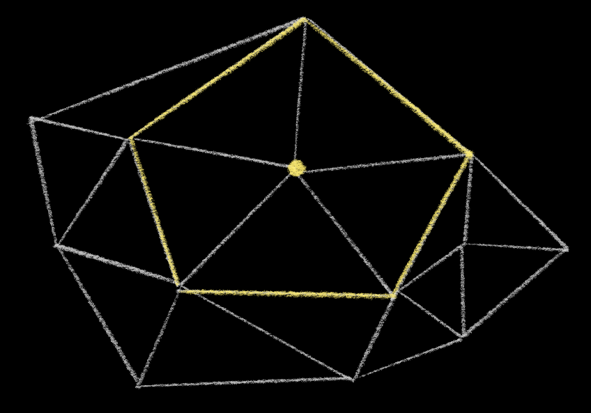
Whenever you add a new point, and connect it to the points of its enclosing triangle or quadrangle, you’ll have a point at the middle of a spoke. Like this:
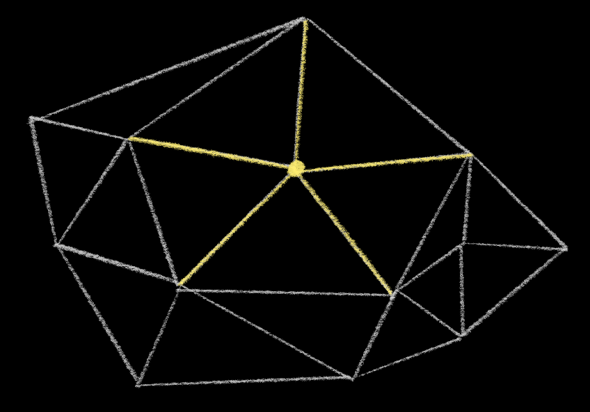
All of those newly created edges are already fine. We don’t have to check them. But we do have to check the edges adjacent to them – the edges that form a ring around the newly inserted point.
Whenever you flip an edge, you make this ring bigger, effectively adding two new segments to the ring.
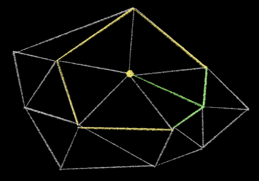
You then have to check those new edges. But notice that they’re still a part of the same ring! And in fact as you flip these edges, they will add new segments to the ring as well.
So you don’t need to store a list of “dirty edges” or recurse to clean up all of these edges. You can just store a specific edge on the ring, check it, and then either move “forward” (if the edge passed) or “backwards” (if you had to flip it).
So the number of edges that you have to check depends on the number of triangles that have the newly inserted point as one of their corners. In the worst case this means means doing O(n) work, but on average across every point insertion this will net out to constant time, apparently, although I can’t find a proof of that.15 But we’re already doing worst-case O(n) work to find the triangle, so the total runtime of the algorithm remains O(n2).
Easy! Okay. Which brings us to the last question: what do we do about the “infinite bounding triangle?”
There is no triangle you can construct that will be “big enough” to pass for infinite when we do the point-in-circle test – as three points get closer to being colinear, the radius of the circle they define will approach infinity – so we just won’t do the point-in-circle test. Whenever a point on our boundary triangle is involved, we’ll instead check a series of conditions:
-
If the edge in question is a boundary edge, do not flip it. This one is easy so I’m not going to draw it for you.
-
If the edge contains a boundary vertex, flip it, unless doing so would create an inside-out triangle.
- If an edge separates our newly inserted point from a boundary vertex, do not flip it.

That’s it! Those conditions will give you answers consistent with the answers you would get if your boundary vertices really were infinitely far from the rest of your points. Now all you need to do is to construct a triangle large enough to contain all of your points so that your “point in triangle” test works correctly, and you’re done. (If you don’t know all your points ahead of time, you can make any triangle and resize it as you learn points.)
are we there yet
Yes! We did it. That’s the algorithm. And the data structure. Two for the price of one.
Now that you understand how it works, in far more detail than you ever wanted to, let’s watch the visualization again. I’m excluding the boundary triangle this time so we can zoom in a bit and just bask in the triangular glow.
Well, that’s it. From here it’s a short, linear-time jaunt to computing the Voronoi diagram, the Gabriel graph, and probably some other interesting stuff. But that’ll have to wait for the next post.
Speaking of next posts, if you enjoyed this one, don’t forget to…
No. I can’t actually say it.
-
You might be wondering why you would want to construct a Voronoi diagram in the first place, to which I can only respond: why wouldn’t you? They’re so cool! ↩︎
-
I googled this phrase before I wrote this post to make sure that this actually is real slang. It seems that “smash that like button” is a more common phrase, but I don’t have a like button. Should I have a like button? Is that a thing that people would smash? What is… what are we doing here?
Here, if you really want to smash a like button, you can smash this one:
Did that feel good? Did you enjoy that? ↩︎
-
Actually, what you’re seeing here is not exactly the Gabriel graph – it’s the union of the Gabriel graph and the convex hull, so that the outline of the button is always solid. ↩︎
-
The Delaunay triangulation is not always unique: imagine four points arranged in a square. There are two ways to cut the diagonal, and either choice gives you a valid Delaunay triangulation. But it is only not unique in the case of co-circular points like that, and this randomly generated example doesn’t have any. ↩︎
-
In the same paper, Guibas & Stolfi describe another algorithm – a divide-and-conquer algorithm, kinda like merge-sort – that seems more complex, but is actually a lot simpler to code. Originally I wanted to describe both of these algorithms in this blog post, but, well, come on. This is so long already. ↩︎
-
Fun fact: this pattern of points is called a quincunx. Say it. Quincunx. say it out loud ↩︎
-
Since finding the distance between two points requires taking a square root, you actually compare the square of the distance against the square of the radius. But you knew that. ↩︎
-
Citation needed. The test as I presented it requires a division operation, while the determinant calculation only requires multiplication and addition. We can remove the division by subtracting Az multiplying both sides of the inequality by Nz, but then we need to invert the logic when Nz is negative (which we can do without branching). But I mean… I neither profiled it nor tallied the individual operations, so I won’t try to argue that the plane test is actually faster. Also, like, numerical precision is a thing that computation geometry people worry about? Is the determinant solution more robust in the face of floating-point errors? I don’t know. ↩︎
-
More precisely, the dual is only defined for a particular planar embedding of a graph. There are lots of ways to draw a picture of a graph, and depending on how you draw it, you might end up with a different dual. ↩︎
-
The paper actually describes two versions of the data structure, first a general version, and then a simplified version that only works for orientable manifolds. What does that mean? I have no idea. I’ve never studied topology. Manifolds are a topology thing, right? Also sorry I know I said I wouldn’t say manifold and now I’ve said it a bunch. ↩︎
-
For a less straightforward representation, I was able to find some code on Stolfi’s university homepage that uses a more space-efficient representation. Paraphrasing slightly:
typedef char * quad_edge_ref;

typedef struct {
    quad_edge_ref next[4];
    void *data[4];
} quad_edge;
The idea here is that a
quad_edge_refis really a pointer to the interior of aquad_edge– anywhere from 0 to 3 bytes from the struct’s base address – and you use bitmasking operations on the pointer to identifymy_indexand to compute the actual base address:// 32 bits ought to be enough for anybody quad_edge_ref *rot(quad_edge_ref edge) { return (edge & 0xfffffffcu) + ((edge + 1) & 3u); } quad_edge_ref next(quad_edge_ref edge) { return ((quad_edge *) (edge & 0xfffffffcu))->next[edge & 3u]; }So it only works if you know how your struct is aligned, and the size of your pointers, and… look maybe this sort of thing could fly in 1985 but I will speak no more of it here. ↩︎
-
Assuming the points of your triangle are defined in counter-clockwise order in the first place. If you think of triangles as being clockwise to begin with, then everything is backwards. Gosh winding order is confusing. ↩︎
-
“Computing Dirichlet tesselation in the plane,” 1977. ↩︎
-
There is an even more clever but much more complicated triangle traversal algorithm that works in logarithmic time by building up something called the “Delaunay tree.” It was first described by Boissonnat & Teillaud in their 1989 paper “On the randomized construction of the Delaunay tree.” It’s conceptually very simple, but I’m not going to explain it because just look at how long this blog post is already. There is a decent overview of it starting on page 46 of this PDF. ↩︎
-
I assume because you can calculate the average number of edges incident to each vertex and that is going to be some small finite number that doesn’t depend on the number of vertices. Like some kind of Euler’s formula for Delaunay triangulations. But I don’t know. I’m sure the proof is out there, somewhere, but I am too tired to look any further. ↩︎